Discovering new phenomena in particle physics, like the Higgs boson, involves the identification of rare signals that can shed light into unanswered questions about our universe. At the Large Hadron Collider (LHC), particle collisions produce vast amounts of data. In this blog post, I explain a project I’m developing for the Google Summer of Code 2024, under the Machine Learning for Science (ML4SCI) organization. I am developing a Lie-Equivariant Quantum Graph Neural Network (Lie-EQGNN), a quantum model that not only is data efficient, but also has symmetry-preserving properties from any arbitrary Lie algebra that can be learned directly from the data. Given the limitations by noise of current quantum hardware, efficiently designing new parameterized circuit architectures is crucial. This blog post highlights an overview of the project. Aiming for the best intuitive explanation, the sections are split into five parts:

• Introduction
• Jet data
• Group theory review
• A primer on quantum/classical graph neural networks.
• Invariant-equivariant machine learning.

Introduction

The story of symmetries and machine learning goes a long way, back to Minsky and Papert. They showed that if a neural network is invariant to some group, then its output could be expressed as functions of the orbits of the group. In recent years, the field of Geometric Deep Learning was born, and it posits that in spite of the curse of dimensionality, the huge success of deep learning can be explained by two main inductive biases: symmetry and scale separation. By leveraging inherent symmetries in the data, the hypothesis space is effectively reduced, models can become more compact, and requiring less data for training - attributes that are particularly critical for quantum computing, given the current hardware limitations.

In particle physics, symmetries underpin the fundamental laws governing the interactions and behaviors of subatomic particles: the Standard Model (SM), for example, is built upon symmetry principles such as gauge invariance, which dictate the interactions between particles and fields.

Recognizing the intertwined nature of symmetries and deep learning, a plethora of models have been developed that are invariant to different groups. Convolutional neural networks (CNNs), for example, which have revolutionized computer vision, are naturally invariant-equivariant to image translations. Transformer-based language models, on the other hand, exhibit permutation invariance. These architectures, when provided with appropriate data, are capable of learning stable latent representations under the action of their respective groups. An interesting question to be explored in quantum machine learning is the use of symmetries, especially in particle physics, which is replete with exotic symmetries. Quantum computers may have a unique advantage in this regard, as they can potentially capture quantum correlations more naturally and efficiently than classical computers. This can open the door to more accurate and insightful models that can better handle the complexities of particle interactions in huge datasets. The caveat is that symmetry is often corrupted by noisy observations, so imposing exact units of equivariance can be suboptimal. We propose to machine learn the Lie algebras behind particle observables, instead of imposing strict symmetry constraints. For this, we aim for three steps in this project:

• Symmetry discovery
• Invariant metric extraction
• Lie-Equivariant Quantum Graph Neural Network (Lie-EQGNN)

Jet data

In this work, we consider the task of determining whether a given jet was originated by a quark or a gluon, given its final state measurements. This is known as jet-tagging. For this, our dataset is constituted of point-clouds, which means that each jet is represented as a graph $\mathcal{G} = \{\mathcal{V,E}\}$, which is a set of nodes and edges, respectively. This is the natural data structure used by Graph Neural Networks [1].

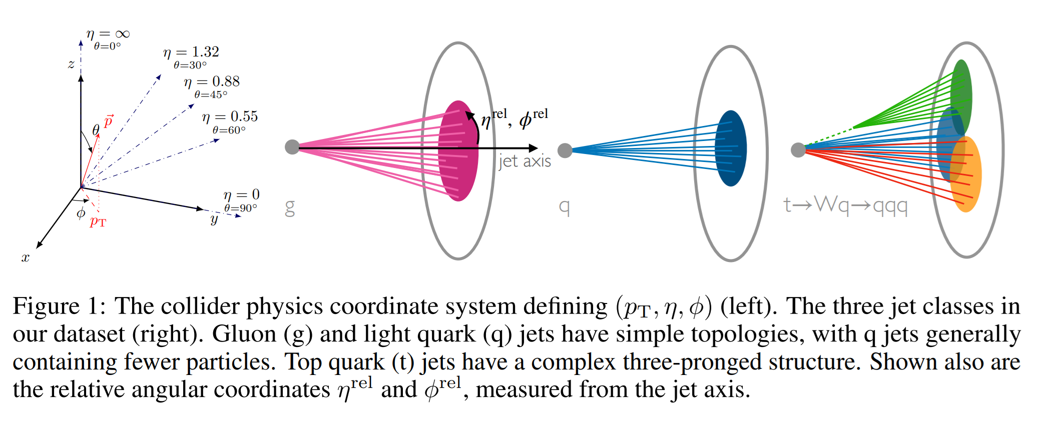
In a typical jet dataset, each node has the transverse momentum $p_T$, rapidity $\eta$, azimuthal angle $\phi$ and some other scalar like particle $ID$/mass - which identifies the particle measured in a multiplicity bin - as its features. Generally, the number of features is always constant, but the number of nodes in each jet may vary.

Group theory review

Symmetries are mathematically represented by algebraic structures called groups. Formally, a group \(\mathcal{G}\) is a set endowed with a binary operation $\cdot$ $: \mathcal{G} \times \mathcal{G} \rightarrow{\mathcal{G}}$, such that:

• $a\cdot (b \cdot c) = (a\cdot b) \cdot c, \forall a, b, c \in \mathcal{G}$ (associativity)
• $\forall g \in \mathcal{G}, \exists$ $I$ such that $g\cdot I = I\cdot g$ (existence of the neutral element)
• $\forall g \in \mathcal{G}, \exists$ $g^{-1}$ such that $g\cdot g^{-1} = g^{-1}\cdot g = I$ (the inverse element always exists)

A Lie group is a continous group endowed with a topology. Specifically, it is a differentiable manifold $M$ that is also a group, and the operations of multiplication and inversion are also smooth maps. For example, all $2D$ rotations can be represented by a parameterized rotation matrix:

In high energy physics, particles moving in a laboratory at velocities neighboring the speed of light, like at the LHC, are described by special relativity. Its fundamental idea is that the laws of physics are the same for all observers in different inertial frames. Mathematically, the transformations between two inertial frames of reference are described by the so-called Lorentz group, mathematically represented as $O(1,3)$. Typically, one restricts the frames to be positively space-oriented and positively time-oriented, which gives rise to a subgroup called the proper orthochronous Lorentz group, or $SO^{+}(1,3)$ - but often just referred to as the Lorentz group, where its canonical generators representations are:

1. Rotation Generators $L^{ij}$:

1. Boost Generators $L^{0i}$:

This is one well-known symmetry group of special relativity, and our idea is to build some parameterized circuit equivariant to this group (or any we wish to discover from experimental data).

Machine-learned symmetries

Setup and notations

Before diving into machine-learned symmetry discovery [2], we’ll equip ourselves with basic notations used throughout this post. Our starting point is a labeled dataset containing $m$ samples of $n$ features and a target label $y$:

in the machine learning realm, a dataset is just an $m\times n$ matrix (usually called a dataframe), where $m$, the number of rows, indicates the number of samples, and $n$, for the columns, the number of features. In this way, a given feature vector $x$ can be written as:

Invariance

Any symmetry is a transformation that leaves some property invariant, ie: rotations, which are length preserving. Formally, we say that we want to learn some transformation $f: \mathbb{R}^{N} \rightarrow \mathbb{R}^{N}$ that leaves some property given by a function $\mathbb{\phi}(x)$ invariant. From now on, we call $\mathbb{\phi}(x)$ an oracle. Such an oracle can be known numerically or analytically, the latter being the case of a particle theorist that wishes to discover the underlying group, for example, working on a new lagrangian beyond the standard model (BSM) that has a new invariant, and wishes to discover what is its underlying group. In the former case, which is the common scenario in data science, one first has to build $\phi$, usually in the form of a neural network, and then train it using some regression method. From a machine learning point of view, either numerical or analytical, the oracle is just a black box that ingests a vector and tells us the property we want to know - the Euclidean norm, the Minkowski norm, etc. Learning a symmetry, then, means that we aim to find some $f(x)$ such that:

where $f$ can be modeled as a classical $1$-hidden layered neural network, or as a matrix. The invariance under $f$ can then be enforced by

which is basically a mean-squared error (MSE) that penalizes the model for learning any transformation that violates the oracle.

Infinitesimality

Ultimately, $f$ is a machine-learned Lie algebra basis, meaning that it is a set of matrices that transform the data through the exponential map. To ensure that $f$ is a Lie algebra generator, we consider infinitesimal transformations $\delta \mathcal{F}$ in the neighborhood of the identity transformation $\mathbb{I}$:

where $\mathbb{G}_{\mathcal{W}}$ is our neural network parameterized $\mathcal{W}$, and $\epsilon$ is an infinitesimal parameter (in practice, we take it to be a small number of the order of $10^{-5}$).

Orthogonality

In order to make the set of generators ${J_{\alpha}}, \alpha = 1, 2, …, N_{g}$, found in the previous step maximally different, an additional orthogonality term to the loss function is introduced:

where the index $p$ runs over the individual NN parameters $W(p)$.

Closure

In order to test whether a certain set of distinct generators ${J_{\alpha}}, \alpha = 1, 2, …, N_{g}$, found in the previous steps, generates a group, we need to check the closure of the algebra. This can be done in several ways. The most principled way would be to minimize

with respect to the candidate structure constant parameters $a_{[\alpha\beta]\gamma}$, where the closure mismatch is designed by

The invariant metric

Once the machine learned generators $L$ are found through the steps to be described here, we can extract the invariant metric tensor $J$ to further build invariant features, effectively baking the symmetries into our Quantum Graph Neural Network (QGNN). To do so, we can solve for:

Numerically, a small push from zero is enough to avoid getting the trivial solution $J = 0$:

The proof for this equation can be found in [3]. The code below implements this procedure and was kindly given by the authors:

# assuming you have the Lie generators stored under 'data'.
L = torch.load('data/top-tagging-L.pt')
a = 0.05
lr = 1.0
J = torch.randn(3, 3, requires_grad=True)
optimizer = torch.optim.LBFGS([J], lr=lr)

losses = []

def closure():
    optimizer.zero_grad()
    loss = 0.0
    for j in range(L.shape[0]):
        Lj = L[j]
        loss += torch.sum(torch.square(Lj.transpose(0, 1) @ J + J @ Lj))
    loss -= a * torch.linalg.norm(J)
    losses.append(loss.item())
    loss.backward()
    return loss

for i in range(1500):
    optimizer.step(closure)
    # if i <= 1000:
    #     scheduler.step()
print(J)

Classical Graph Neural Networks

Graph Neural Networks (GNNs) are a class of neural networks designed to operate on graph-structured data. Unlike traditional neural networks that work on Euclidean data such as images or sequences, GNNs are capable of capturing the dependencies and relationships between nodes in a graph. The fundamental idea behind GNNs is to iteratively update the representation of each node by aggregating information from its neighbors, thereby enabling the network to learn both local and global graph structures.

Mathematically, a GNN can be described as follows: Let $( G = (V, E) )$ be a graph where $( V )$ is the set of nodes and $( E )$ is the set of edges. Each node $( v \in V )$ has an initial feature vector $( \mathbf{h}_v^{(0)} )$. The node features are updated through multiple layers of the GNN. At each layer $( l )$, the feature vector of node $( v )$ is updated by aggregating the feature vectors of its neighbors $( \mathcal{N}(v) )$ and combining them with its own feature vector. This can be expressed as:

where $( \mathbf{W}^{(l)} )$ and $( \mathbf{W}_e^{(l)} )$ are learnable weight matrices, $( \sigma )$ is a non-linear activation function, and $( \mathcal{N}(v) )$ denotes the set of neighbors of node $( v )$. This process is repeated for a fixed number of layers, allowing the network to capture higher-order neighborhood information.

The final node representations can be used for various downstream tasks such as node classification, link prediction, or graph classification.

Quantum Graph Neural Networks

Now that we know that classical GNNs aim to learn a lower-dimensional topologically preserving representation of our graph, we turn to quantum graph neural networks [4] (QGNNs). One possible approach for them is to first find some Hamiltonian that can describe the nodes, or qubits, in our graphs, and also their interactions, or edges. We can achieve this by considering the transverse-field Ising model, originally introduced to study phase transitions in magnetic systems, which is given by:

where $\theta = \{\mathcal{W}, \mathcal{M} \}$, $E$ is the set describing all pairs of nodes, $\mathcal{W_{ij}}$ is a learnable edge matrix, and the coupling term represents interactions between nodes by two coupled Pauli-Z operators $Z_i$ and $Z_j$, respectively, acting on nodes $i$ and $j$. The first-order terms are used to describe node weights, where each $\mathcal{M}_{i}$ is a learnable feature representing the node weight, and they are essentially measuring the energy of individual qubits.

Given the Hamiltonian, we wish to convert it to a unitary so it can be implemented on a quantum computer. Recalling the time-evolution operator, we can achieve this through:

\begin{equation} U = e^{-itH}, \end{equation}

which, for the Ising Hamiltonian, becomes:

Unfortunately, this is a hard ansatze to be implemented on quantum hardware, in general. With the Trotter-Suzuki decomposition [5], however, it becomes feasible by the approximation:

and hence, the final form of the unitary operator to be implemented on quantum hardware is given by: \(\begin{equation} \hat{U}_{\mathrm{QGNN}}(\boldsymbol{\eta}, \boldsymbol{\theta})=\prod_{p=1}^P\left[\prod_{q=1}^Q e^{-i \gamma_{p q} \hat{H}_q(\boldsymbol{\theta})}\right] \end{equation}\)

Where $\gamma_{pq}$ can be thought of as an infinitesimal parameter (small number, in practice).

Invariant-equivariant machine learning

The idea of symmetry-preserving behavior in machine learning is crucial. As the hypothesis space is effectively reduced, learning becomes easier. Also, models that incorporate geometric information as an inductive bias are naturally data-efficient, and the common practice of using augmentation for training can be drastically reduced (or even eliminated). For QML, given the limited qubits, this is a fundamental property that we want in our models.

As illustrated above, given some function $f: \mathcal{X} \rightarrow \mathcal{Y}$ (for example, $f$ could be a neural network, $\mathcal{X}$ the input space, and $\mathcal{Y}$ a latent space) and some group $G$ that acts on both $\mathcal{X}$ and $\mathcal{Y}$, then $f$ holds the desirable property of equivariance if $\forall g \in G, (x, y) \in \mathcal{D}, T_y (g) y = f(T_x (g) x)$. For brevity of notation, we just write it as:

From this, we can see that invariance is a special case of equivariance where $f(g\cdot x) = f(x)$, that is, $T_y (g) = \mathbb{I}$, so every group element acting in the space of $\mathcal{Y}$ gets mapped to the identity. To introduce invariance in the architectures, one must first find the group $G$ that explains the underlying transformations on the data. In our case, these are Lie groups.

Equivariant Quantum Neural Networks

Given some group $\mathcal{G}$, the first way to achieve equivariance [6] is to have a quantum neural network of the form $h_{\theta} = Tr[\rho \tilde{O}_{\theta}]$ such that:

To see why, we need to observe that the trace is cyclical, so:

Essentially, we are using the Heisenberg picture, where we apply the time evolution to the measurement operator instead of the initial quantum state. When the observable is included in the commutant of $\mathcal{G}$, we can see how invariance is achieved.

The challenge with this approach is that it only works for finite-dimensional and compact groups, like $p4m$, $SO(3)$, etc. The Lorentz group is known to be continuous and non-compact, so it has no finite-dimensional unitary representation. Hence, the approach above is of no use for us. Hopefully, there is another way: instead of baking equivariance directly into the ansatze, we’ll do it in the feature space and in the message passing function.

Similarly to LorentzNet, for standard jet tagging approach, our input is made of $4$-momentum vectors and any associated particle scalar one may wish to include, like color and charge. In fact, in this project, we start with the traditional LorentzNet architecture, but two modifications are made: first, the invariant metric can be extracted from the machine learned algebra; secondly, the $\phi_e, \phi_x, \phi_h$ and $\phi_m$ - classical parts modeled as classical multilayer perceptrons in Lorentznet, are substituted by quantum counterparts, that is, variational circuits. Below we show how invariance-equivariance is preserved under this modification.

Lie Equivariant Quantum Block (LEQB)

LEQB is the main piece of our model. We aim to fundamentally learn deeper quantum representations of $|\psi_{x}^{l+1}\rangle$ and $|\psi_h^{l+1} \rangle$ from $|\psi_{x}^{l} \rangle$ and $|\psi_{h}^{l}\rangle$, where:

where $\mathcal{U_{x^{l}}}, \mathcal{U_{x^{l+1}}}, \mathcal{U_{h^{l}}}, \mathcal{U_{h^{l+1}}}$ are all parameterized standard gate unitaries, or variational circuits. Note that $x^{l}$ are the observables and $h^{l}$ are the particle scalars when $l=0$, but $x^{l} = \langle \psi_x | \mathcal{M} | \psi_x\rangle$ and $h^{l} = \langle \psi_h | \mathcal{M} | \psi_h\rangle$ for $l > 0$, where $\mathcal{M}$ is some measurement operator.

Theoretical analysis

Let’s start with the following proposition:

The coordinate embedding $x^{l} = {x_1^{l} , x_2^{l} , \dots , x_n^{l}}$ is Lie group equivariant and the node embedding $h^{l} = {h_1^{l} , h_2^{l}, \dots , h_n^{l}}$ - representing the particle scalars - is Lie group invariant.

To prove it, let $Q$ be some Lie group transformation. If the message $m_{ij}^{l}$ is invariant under the action of $Q$ for all $i,j,l,$ then $x_{i}^{l}$ is naturally Lie group equivariant since:

where $Q$ acts under matrix multiplication. The equation above means that acting with $Q$ from the outside is the same as acting with $Q$ from the inside - directly into the node embeddings from the layer before. Then, for the invariance of $m_{ij}^{l}$, since the norm induced by the extracted metric is invariant under the action of $Q$, it holds that $||x_{i}^{0} - x_{j}^{0}||^2 = ||Q\cdot x_{i}^{0} - Q\cdot x_{j}^{0}||^2$, and $\langle x_{i}^{0}, x_{j}^{0} \rangle = \langle Q\cdot x_{i}^{0}, Q\cdot x_{j}^{0} \rangle$. Since $m_{ij}^{l+1} = \phi_e(h_i^{l}, h_j^{l}, ||x_{i}^{l} - x_{j}^{l}||^2, \langle x_{i}^{l}, x_{j}^{l} \rangle)$, and the norm and the inner product are already invariant, we just have to show that $h^{l}$ is also invariant, since:

For layer $l=0$, $h_{i}^{l}$ is already invariant (since it contains information only about the particle scalars). Then, $m_{ij}^{l+1}$ will be invariant, since all of its inputs are also invariant, and we follow the same logic for $x_{i}^{l+1}$. Given that these properties of $x,h,m$ hold for the first layer and the next, we reach the conclusion recursively.

Having a quick glance at the discussion we had about groups, equivariance, particles and quantum machine learning, we are getting a hint that the marriage between Physics and symmetries is actually deep. Indeed it is! To quote Philip Anderson, who won the 1977 Nobel prize “for their fundamental theoretical investigations of the electronic structure of magnetic and disordered systems”:

It is only slightly overstating the case to say that physics is the study of symmetry.

Results

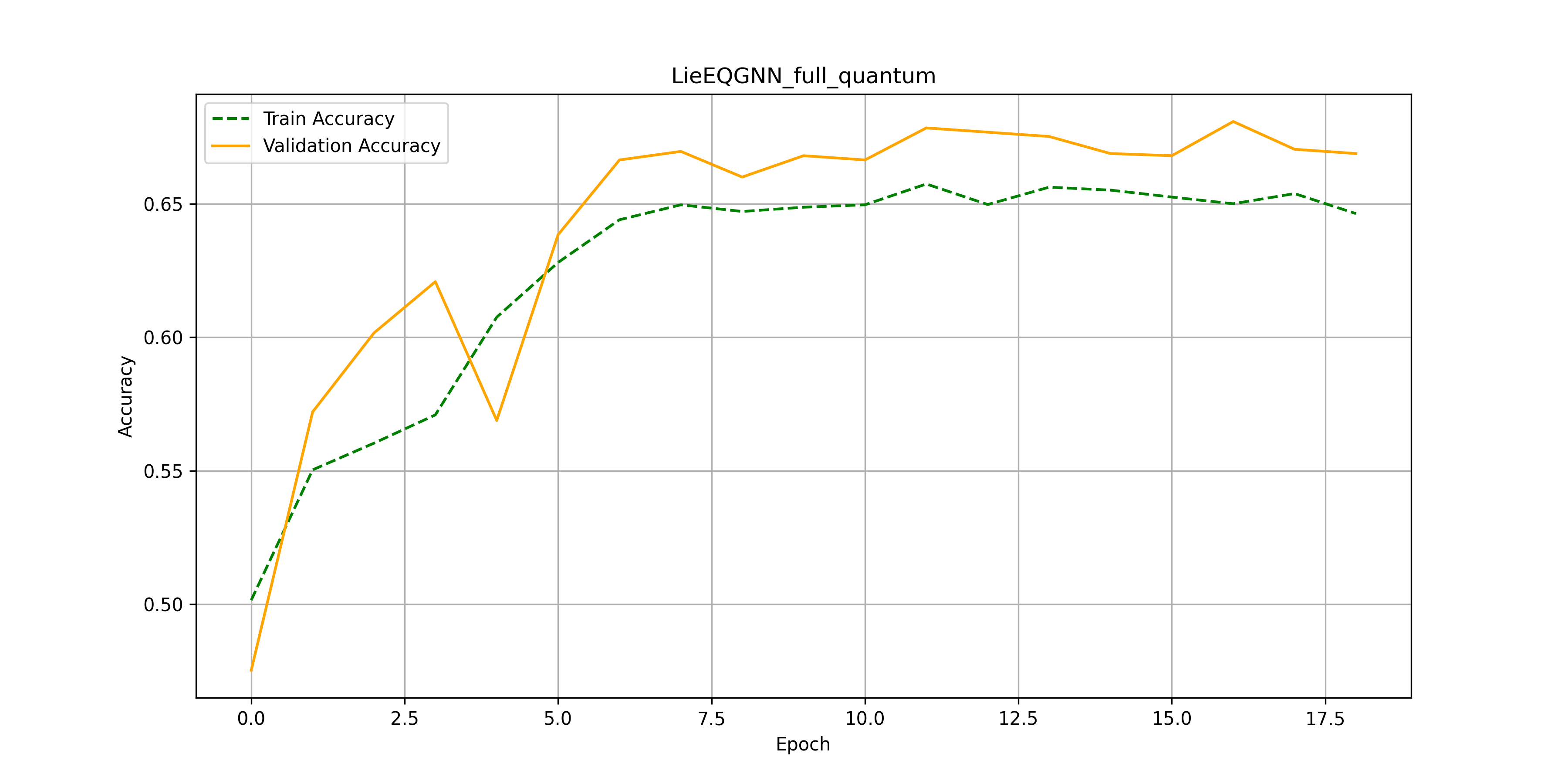
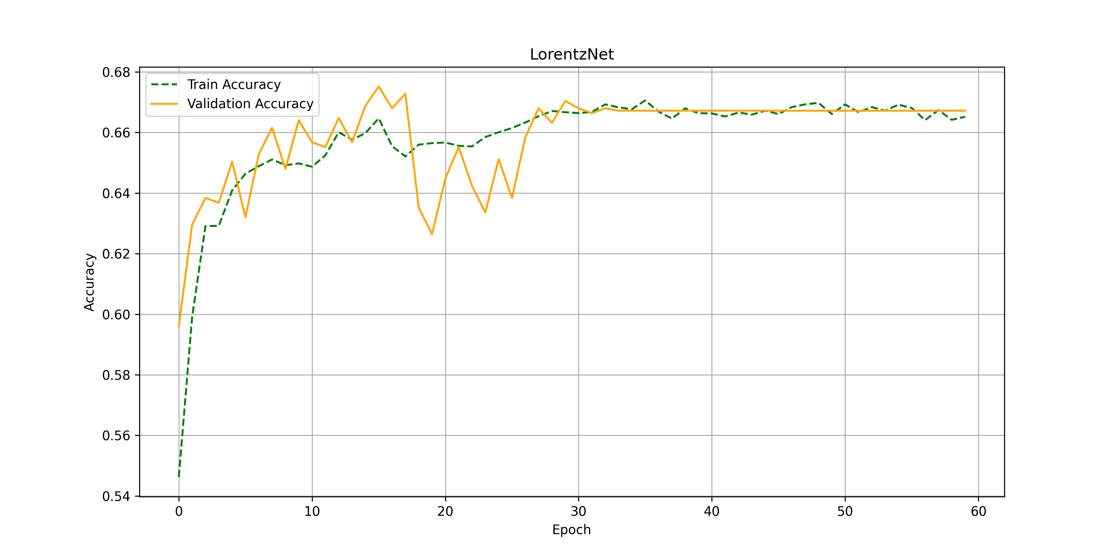
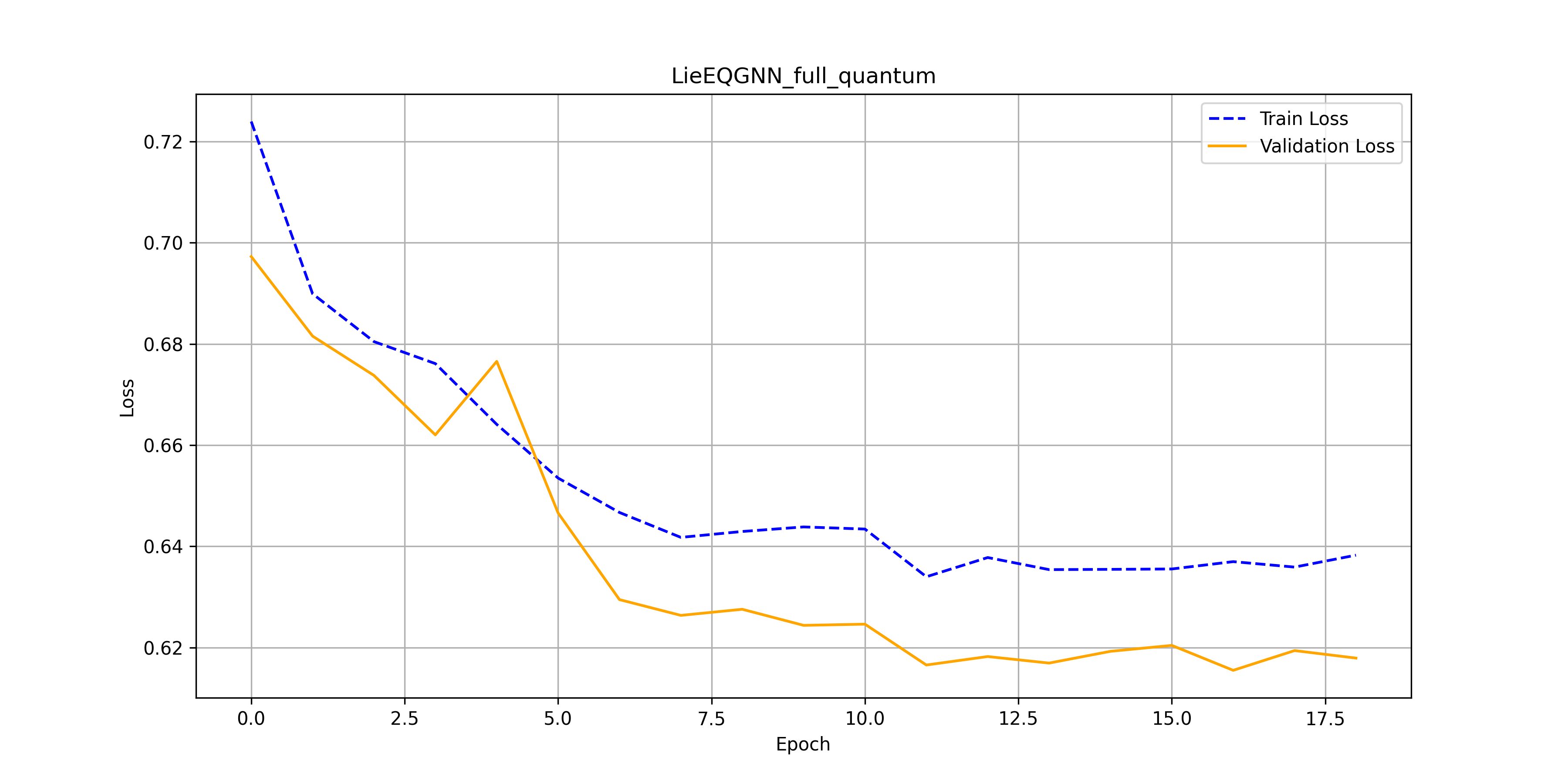
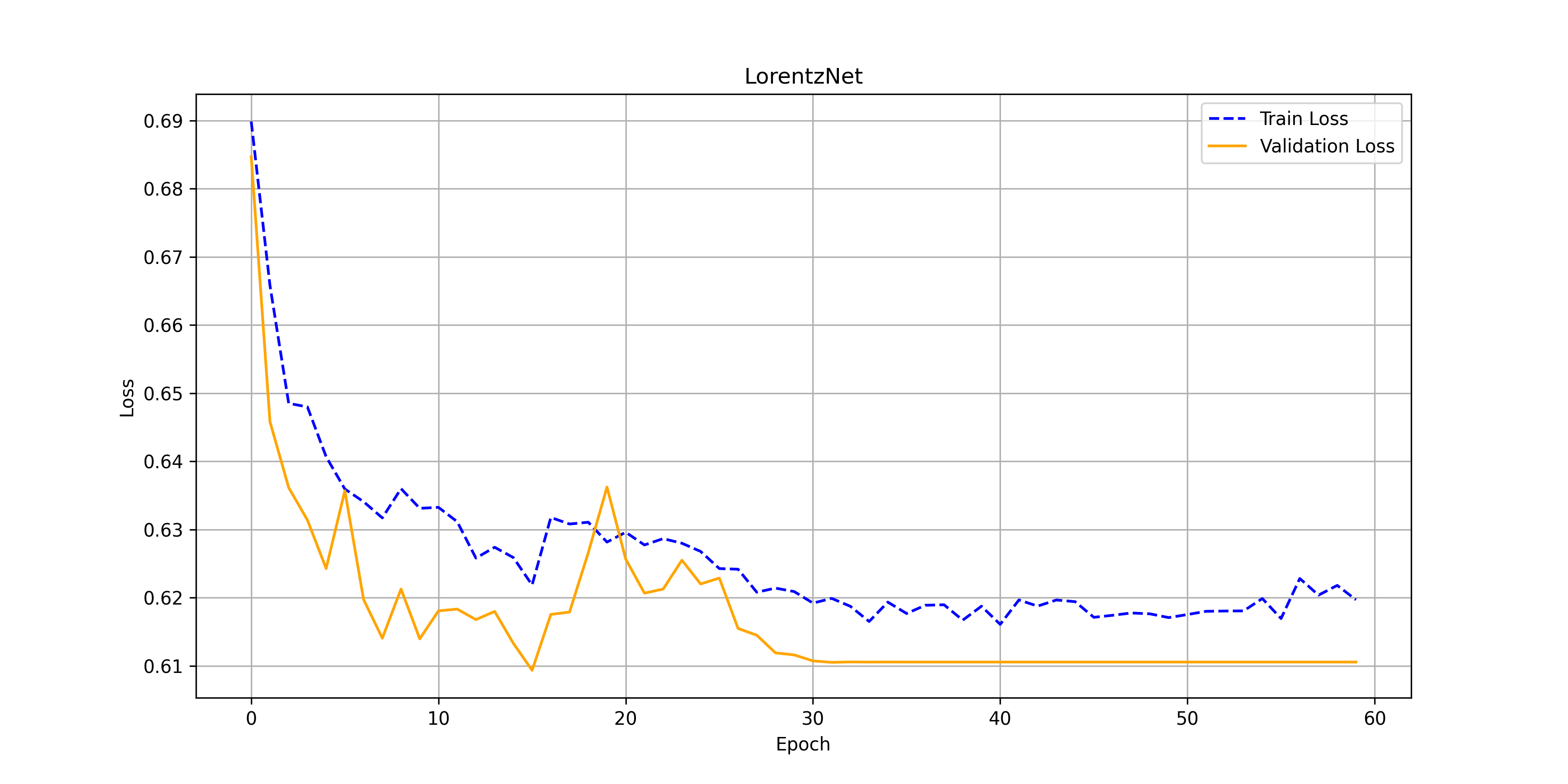
After substituting $\phi_e, \phi_x, \phi_h$ and $\phi_m$ for parameterized circuits, below we can find the results (accuracy and losses over training epochs) achieved on quarks vs gluons data.

Code

All the code is available on https://github.com/jogisuda/Lie-EQGNN

References

[1] Shlomi, Jonathan, Peter Battaglia, and Jean-Roch Vlimant. “Graph neural networks in particle physics.” Machine Learning: Science and Technology 2.2 (2020): 021001.

[2] Forestano, Roy T., et al. “Deep learning symmetries and their Lie groups, algebras, and subalgebras from first principles.” Machine Learning: Science and Technology 4.2 (2023): 025027.

[3] Yang, Jianke, et al. “Generative adversarial symmetry discovery.” International Conference on Machine Learning. PMLR, 2023.

[4] Verdon, Guillaume, et al. “Quantum graph neural networks.” arXiv preprint arXiv:1909.12264 (2019).

[5] Naomichi Hatano and Masuo Suzuki. Finding Exponential Product Formulas of Higher Orders, page 37–68. Springer Berlin Heidelberg, November 2005.

[6] Nguyen, Quynh T., et al. “Theory for Equivariant Quantum Neural Networks” PRX Quantum 5.2 (2024): 020328.